$ Implementing Turbo Codes in Python - Updated on 10/16/18
Overview
Turbo codes are a class of error correction codes built so that the receiver can attempt to reconstruct the original message if it was corrupted over a noisy channel. As an example, they are used in 3GPP LTE (4G) for cellular communications.
Turbo codes have become essential to certain wireless communication systems due to their performance. It is possible to operate near the channel capacity with long enough codes and maintain reasonable decoding complexity.
The objective of this tutorial is to give a quick description of the algorithms that make up the turbo encoder and decoder, and focus on a simple implementation in Python. I will state the algorithm in its non-probabilistic form, and leave the reader to the references to learn more about the theory and maths. Often, those references do not provide enough details or advisories to help with implementations.
I do not delve into puncturing, which optional from the decoder’s point of view, and helps increase the rate of the code (e.g. from R=1/3 to R=1/2).
Turbo Encoders
In this example, a rate 1/3 turbo code encoder consists of two recursive systematic convolutional (RSC) encoders, and an interleaver before the second encoder. The purpose of the interleaver is to ensure the parity bits are mostly independent. Figure 1 provides a simple picture of the encoder setup.
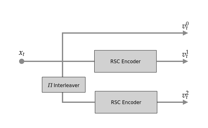
Figure 1: Turbo Encoder Diagram
An individual RSC encoder can be represented by a single segment of a trellis diagram, illustrated by figure 2. The output is determined by the current state and the input bit. Eventually everything is concatenated together where at each output instant you have a tuple with the first systematic bit (original input bit) and the outputs of the two encoders.
The structure of a convolutional encoder (RSC encoder) is made of up memory registers that each hold 1 bit, and some number of modulo-2 adders. In our example, we’re using a simple recursive convolutional code.
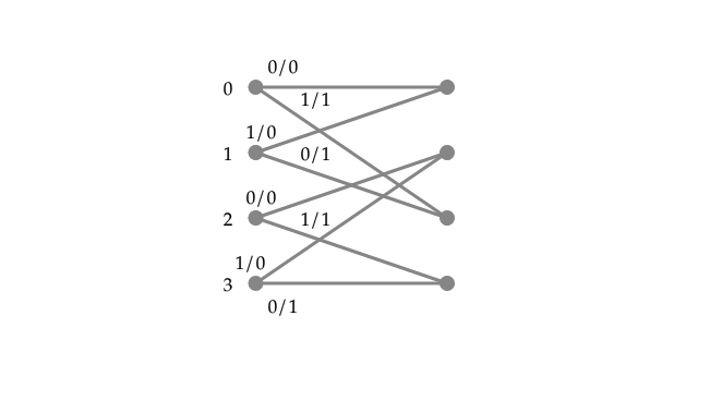
Figure 2: Trellis section which represents a single RSC encoder
The left most numbers represent the state of the encoder, while the binary numbers on each transition represent the input bit / output bit.
My reference implementation of a turbo encoder can be found here.
It is extremely important that the first component RSC encoder terminate at its original state (usually zero), otherwise the turbo decoder will introduce bit errors near the end of the input message and mess up any BER curves.
Single Input Single Output (SISO) MAP Decoder
The maximum a posteriori (MAP) algorithm is the engine in the turbo decoder. The algorithm is also called the Bahl, Cock, Jelenik, and Raviv algorithm (BCJR). Essentially, one is trying to estimate the bit probability conditioned on the received sequence in the decoder. This is the algorithm that makes a SISO decoder.
The SISO decoder is one of two components in a turbo decoder. This is the hardest part of the turbo decoder algorithm, and it suffices to get one decoder working before trying to create the feedback mechanism.
The algorithm is stated as follows:
- Calculate branch metrics based in the input message:
$ s_m $ and $ s_n $ correspond to the state transition that occurred on the trellis. $ c_k^0 $ and $ c_k^1 $ correspond to the input / output bits of the trellis shown in the previous figure 2. $ L_a $ corresponds to the prior (extrinsic) values, which are initialized to zero when the first decoder executes on the first iteration.
- Compute the forward path metrics along the trellis:
- Compute the backward path metrics in the opposite direction on the trellis:
- Compute the Log-Likelihood Ratios (LLRs):
The input vector can be interpreted as a list of tuples with the first value corresponding to the systematic (original) bits, and the other values corresponding to the output codeword bits. In the MAP algorithm, we are trying to determine the likelihood of receiving a particular bit at time \( k \) by using the branch and path metrics to score transitions on the trellis. Only the branch metric calculation requires the input vector, after which the path metrics are calculated recursively using the branch metrics as input.
My implementation of the SISO decoder can be found here.
The Turbo Decoder
The turbo decoder ties together two SISO (MAP) decoders and uses the output of the first to act as extrinsic (prior) information to the second. Figure 3 illustrates how the two decoders are tied together, and it is probably easy to guess the origin of the term turbo: the turbocharger used in automobiles.
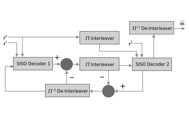
Figure 3: Turbo Decoder Diagram
To further show how a turbo decoder works, figure 4 displays the soft bit outputs after each iteration. One can see how the turbo decoder gains confidence after each computation of the log-likelihood ratios (LLRs). The distance between the soft bit values and the origin grow with every iteration, making the hard decision \( \left( x_t > 0 \rightarrow 1, x_t < 0 \rightarrow 0 \right) \) easier.
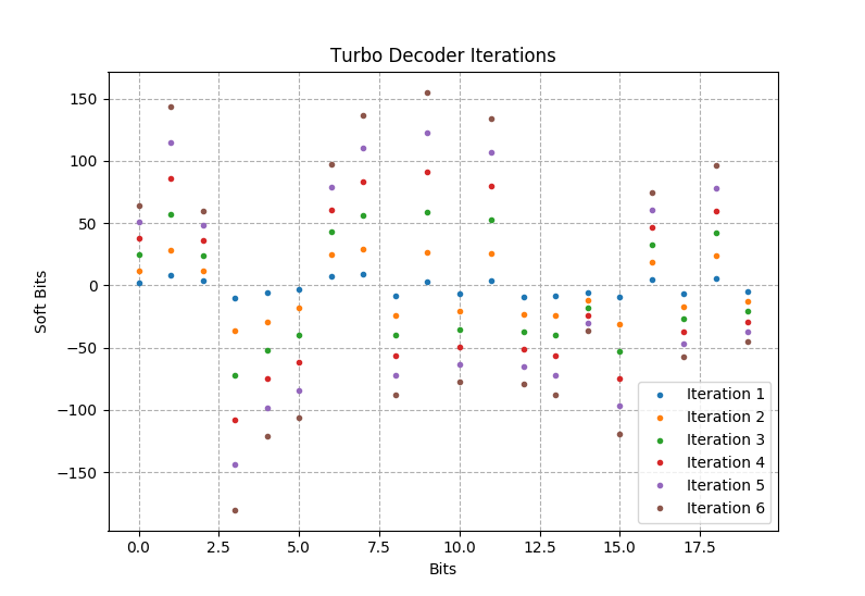
Figure 4
In order to test the turbo decoder over a wide range of signal-to-noise (SNR) ratios, I produced a bit error rate (BER) curve comparing a coded BPSK performance versus an uncoded BPSK signal. One can measure a very large coding gain if a required BER is specified, as shown in figure 5. The number of iterations depends on if the outputs of the SISO decoders agree with each other. This is called the early-exit criterion.
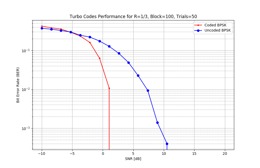
Figure 5
My full reference implementation can be found on my GitHub, along with examples that produced the above results.
References
- Todd K. Moon. Error Correction Coding: Mathematical Methods and Algorithms. Wiley 2005.
- Haesik Kim. Wireless Communications Systems Design. Wiley 2015.
- Wikipedia Article on Turbo Codes.